Metrics At Scale: How to Scale and Manage Millions of Metrics (Part 2)

With businesses collecting millions of metrics, let’s look at how they can efficiently scale and deal with these amounts. As covered in the previous article (A Spike in Sales Is Not Always Good News), analyzing millions of metrics for changes may result in alert storms, notifying users about EVERY change, not just the most significant ones. To bring order to this situation, Anodot groups correlated anomalies together, in a unified alert.

Names Similarity

We’ll start by looking at the ‘Name Similarity’  between metrics. Let’s look at the full procedure for finding name similarity, including how to scale it by using a Locality-sensitive Hashing (LSH) algorithm, and then how it can be modified to other types of similarity.

Metrics are not just numbers, they have names too. Here is an example of a metric:

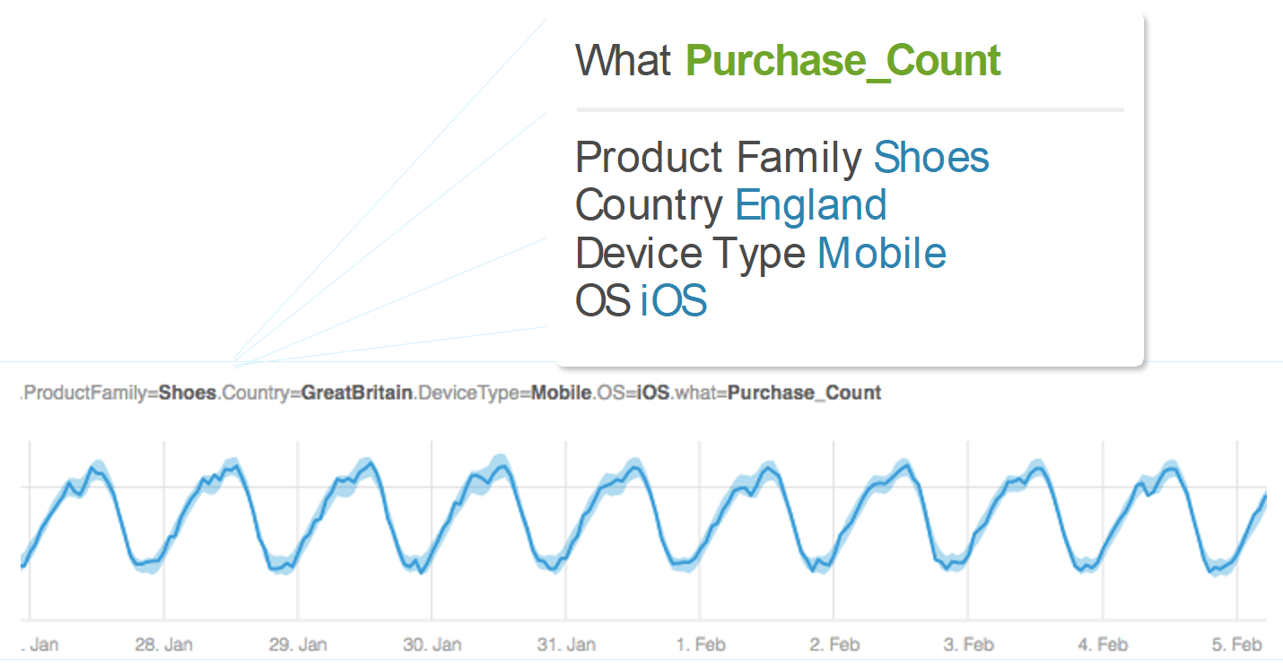
The metric counts the number of shoes purchased by users in England that were using their iOS based mobile devices. The name of the metric describes what it measures, “the purchase count”, and where it was measured: product family, country, device type and operating system. Millions of such metrics may be collected with different measures. These metrics can also be for revenue or price, different products, different countries, or different devices and so on. The names of the metrics are an indication of the relationship shared between them. So, for example, the number of shoes sold to customers in England, who purchased using  their iOS mobile device is probably related to the average price. The similarity between the names of the metrics is a strong indication for the relationship between the metrics.

How can we measure the similarity between two metrics?

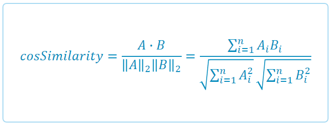
Given two metrics, we will calculate the cosine similarity between their names, by considering the number of shared property/values.

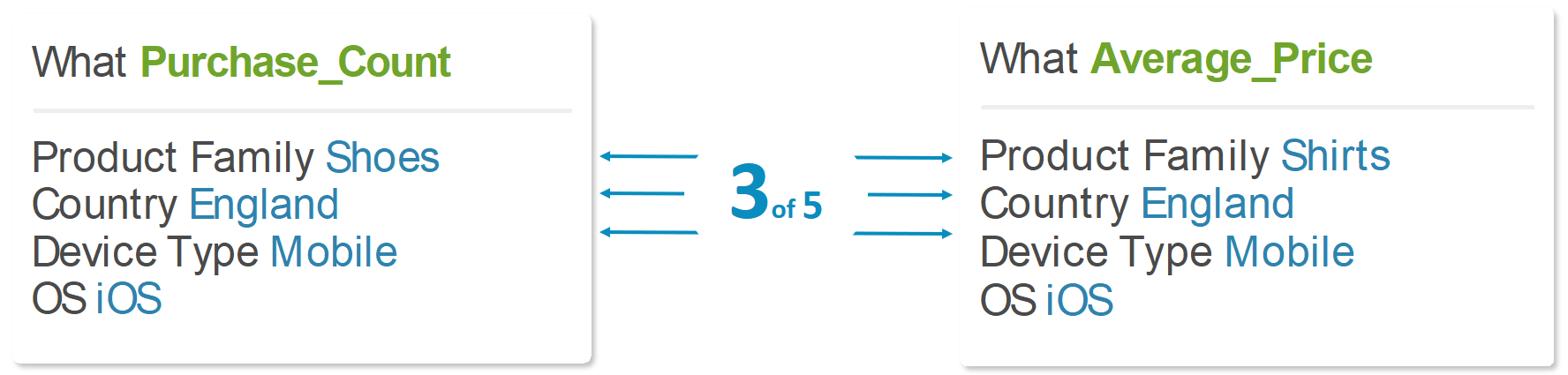
In this example, there are three shared properties: country, device type, and operating system. We divide it by the norms of the vector representation of the metric names (see next section). For example, if each of the above metrics has 5 properties, then the norm of each metric name is √5, and the similarity is 3/(√5⋅√5)=0.6. If the similarity is bigger than a specific threshold, then the two metrics are similar.

Some properties are more common than others. For example, if most of the sales took place in England then Country: England will be very common. The more common properties can influence the similarity score. We want to give less weight to common properties, and more weight to rare properties which can better distinguish the metrics. In order to give weight to the property values, we use IDF (Inverse Document Frequency). The weight of the property value reflects how common it is in all of the metrics. The IDF of the property value is the number of metrics with this property divided by the overall number of metrics, deducting the log of this. The more frequent the property then the lower the weight.

From Metric Name to Vector Representation

Now that we have the weights of all of the property values, each metric name is represented as a vector. First we build a dictionary of all the property values that we have for all our metrics. In our example this dictionary contains: purchase count, average price, product families (shoes and shirts), countries (England) and so on.

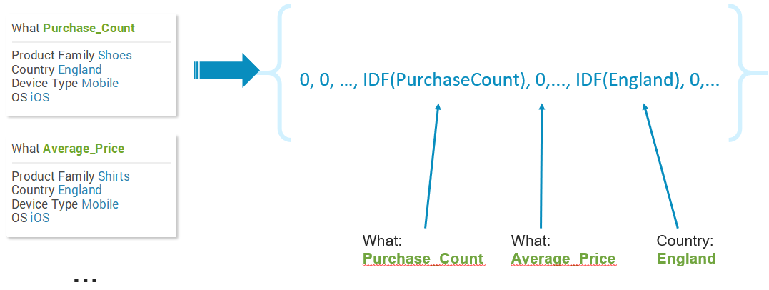
Each metric is converted to a sparse vector representation in the size of the dictionary.

Each property value in the dictionary will have a corresponding entry in the vector. Given a metric name, for each of its property values we put its IDF weight in the corresponding entry of the vector, and for the rest of the vector entries we put zero.

For example,

• Initialize all the vector entries to zero
• For “What”: put the IDF of purchase count in the relevant entry
• For “Country”: put the IDF of England in the relevant entry

Now that we have a sparse vector representation for each of the metric names, calculating the cosine similarity is a simple operation based on the vectors.

Scale is a Big Data Issue

While we know how to calculate similarities between two metrics, a business may have millions of metrics. 1 Million metrics can induce to ≈10¹² pairs, and it is infeasible to compute the similarities between all of them, even using advanced pruning techniques.

One way to overcome this challenge is by using an LSH (Locality-sensitive Hashing) algorithm.

The overall idea of LSH is that every metric is mapped to a hash code. The closer two metrics are, the bigger the probability that their hash codes will be identical. This may sound like magic, but there is a full theory explaining why 2 similar metrics will have the same hash code with high probability. It works only with hashing based on random projection, and the input vectors should be sparse.

All the metrics which are mapped to the same hash code are candidates for being similar. Similarities are calculated only between them, and in Anodot, this process has reduced the computation time by several orders of magnitude.

A summary of the procedure of how we calculate names similarities:

1. Create an ordered dictionary of property values from all our metrics
2. Compute the IDF weight of each of these property values pairs
3. Create the vector representation of each metric as described above
4. Compute the hashes of each of these vectors
5. For each hash group calculate the exact similarities between its members

Watch the full presentation

Presented at O’Reilly’s Strata Data Conference, New York, Sept. 2017