
In our previous article (How to Scale and Manage Millions of Metrics), we looked at correlations in terms of name similarity, but there are other types of similarities that occur between metrics.
Abnormal Behavior Similarities
Metrics can be correlated by their abnormal behavior. When anomalies often appear at the same time in two metrics, we can assume there is a correlation between them.
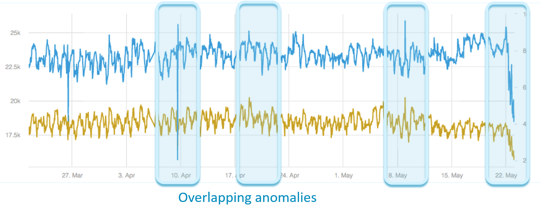
If two metrics are independent, the probability that they will have overlapping anomalies gets lower and lower the more anomalies that they have. This is why it’s important to identify abnormal similarity.
Calculating Abnormal Similarity
The procedure for calculating abnormal similarity is almost identical to the procedure for name similarity, the only difference is in the way that the sparse vector representation is calculated.
How is this done? Anomalies are discovered in each of the metrics for a fixed period, say the last 90 days. The metric is represented in a binary sparse vector in the size of this period, so that whenever the metric is abnormal it is designated by a ‘1’ in this vector and whenever it is abnormal it is designated by a ‘0’.
The next steps are exactly the same as done with name similarity.
The hashes of each of the transformed time series are compared, and for each hash group the exact similarities between its members are calculated.
Another alternative which is applicable for other types of similarities as well, is instead of calculating similarities between each pair in the hash group, a clustering algorithm can be run within each hash group, such as LDA (latent Dirichlet allocation), using the similarity as the distance measure. This is sometimes very useful because groups of similar metrics are often more interesting than just pairs.
Normal Behavior Similarities
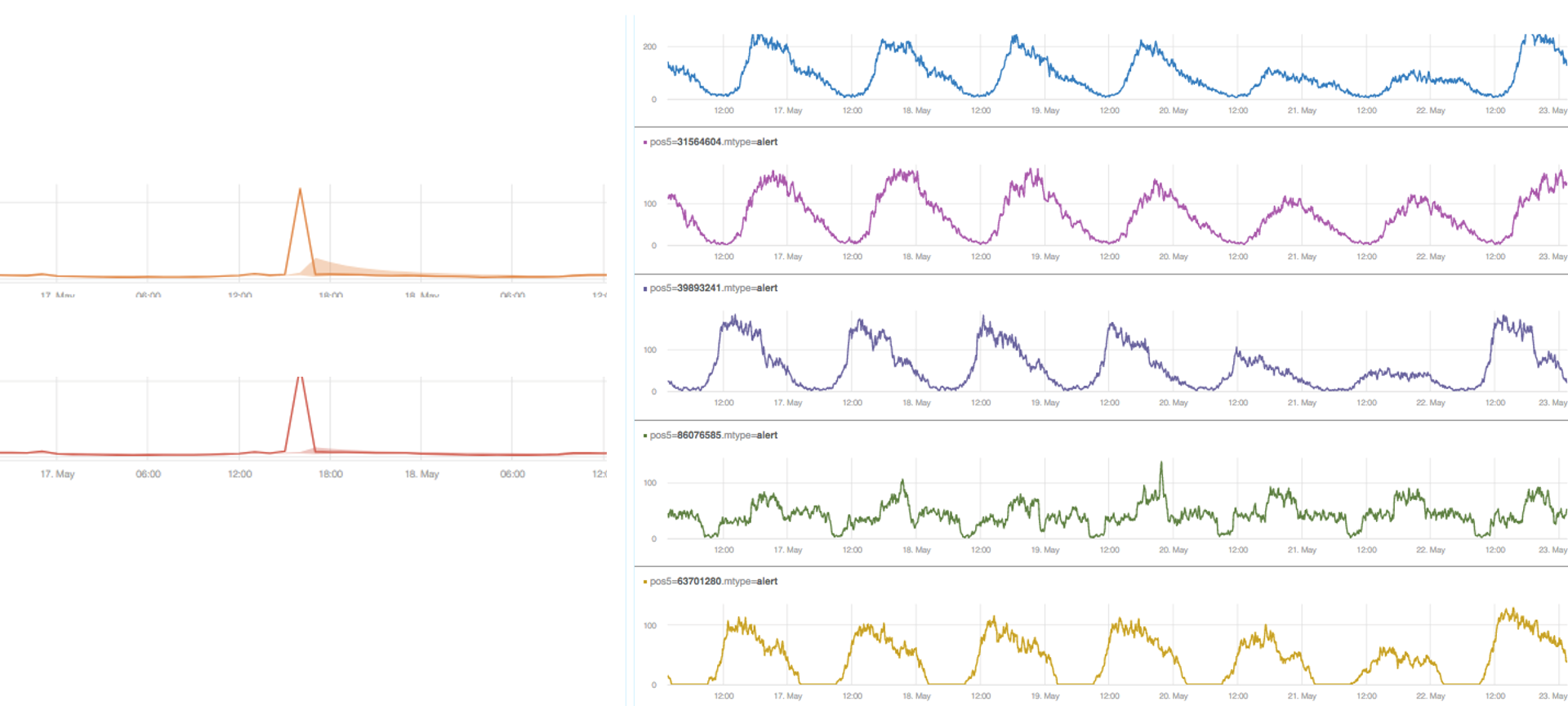
When two metrics behave similarly, and they have similar patterns, then it can be assumed that there is a correlation between them.
By looking at these examples, it can be assumed that the first three metrics and the last one are probably correlated.
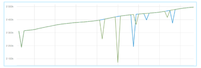
Computing the normal behavior similarities is not so simple. One way to do it is to use various types of linear correlation methods such as Pearson’s correlation, or cross correlation if there is a lag between the metrics. Linear methods are very problematic. They’re very sensitive to trends and to seasonal patterns. Even after removing these using de-trending and de-seasoning techniques, they often don’t work well. They are super sensitive to scale; the two metrics in the following example are very different most of the time.

Over a very small period with extremely high values, they are similar. This small period may totally bias the similarity between them. In this specific example the similarity is almost 0.99, which is very high.
So far, we experimented by using linear methods. Despite tweaking, these always gave results that had either too many false positives or too many false negatives. Another problem is scaling, because by using the original values of the metrics, it’s impossible to avoid high dimensional dense vector representation. For example, 90 days of hourly sampling intervals induced a vector size cardinality of 2160. In order to use LSH (Locality-sensitive hashing) to scale, we must have sparse vector representation or low dimensional representation.
Getting a Sparse or Lower Dimensional Vector Representation
How can we get a sparse or lower dimensional vector representation for each of our metrics?
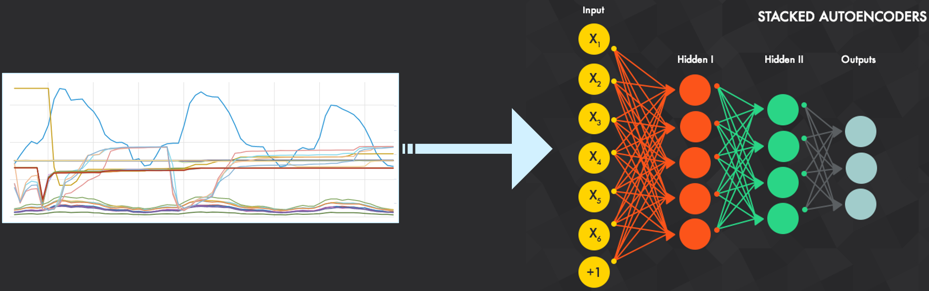
Instead of looking at the metric as a sequence of values, this metric can be looked at as a sequence of patterns. Take this example:
It can be viewed as a sequence of spike, straight line, straight line, straight line, then spikes and so on.
A pattern dictionary can be created, then using a pattern matching engine each metric can be represented by those patterns. Each metric’s original value sequence is converted to a sequence of patterns. This representation is sparse or low dimensional (depending on the implementation). It is amenable to regular clustering and similarity methods. The same procedure that is used for name correlation and abnormal correlation can be used. IDF (Inverse Document Frequency algorithm) can be used to weight the patterns so that common patterns get lower weights and rare patterns get higher weights.
Creating a Pattern Matching Engine
The pattern matching engine is built using deep learning. This entails training a stacked auto encoder with many time series data metrics. The input of the metric is ordered entries (after some preprocessing, including detrending and normalization) and the output is the matched patterns of the metric.
After training the network, the network can be used to convert each of the metrics into their new sparse representation based on patterns. When the metrics have been converted to pattern based representation of each sequence, any similarity procedure can be applied and it can be scaled with LSH.

The Value for Anodot
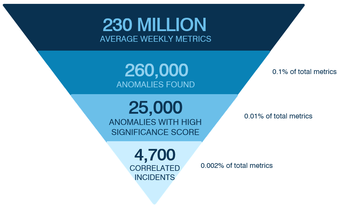
To show the value for Anodot, here are some weekly statistics that we’ve collected.
- Collected: 230 million metrics over the week.
- Detected from them: 260 thousand anomalies
- Found from these that there were significant anomalies with high scores: 25 thousand
- After using the similarity procedure, this was reduced to 4,700 correlated incidents of anomalies.
Taking a look at some other stats, where data was collected for over a month, we calculated:
- ~350 million abnormal correlations [358,543,449]
- ~430 million normal correlation [436,796,325]
- ~370 million name correlations [371,020,643]
- Overall over 1 billion correlations in a month
Summary: Find relationships between different metrics
To summarize, it’s very important to correlate or find relationships between different metrics. This can be used to make order, cluster anomalies. This can reduce the number of incidents of anomalies, and be used to identify and analyze problems or discover opportunities. Knowing the relationship between metrics allows for more accurate prediction and forecasting. For example, knowing that the sales of a product are increasing, we can predict that the sales of another related product will also increase or decrease accordingly.
Part 1: A Spike in Sales Is Not Always Good News
Part 2: How to Scale and Deal with Millions of Metrics
Presented at O’Reilly’s Strata Data Conference, New York, Sept. 2017